previous topic

6.3 Stock Price Dynamics

Here we introduce a model of stock price behavior over time that allows for uncertainty.

The Certainty Case Revisited

In the certainty case, the stock price at the time of the option's maturity, T, equals the future value of the stock price S when continuously compounded at the risk-free interest rate r:

One way to think about this is that the future value is the end result of a dynamic process. That is, the stock price starts at S at the present time 0, and evolves through time to its future value.

The formal expression that describes how the stock price moves through time in the certainty case can be obtained by employing a little calculus:

This says that the rate of change of the stock price over time is proportional to the stock price at time t. The derivation of this representation is provided in Appendix D, topic D.1, Stock Price Dynamics: Certainty Model.

The expression above describes the dynamic stock price process in a world with certainty. Multiplying both sides by dt and rearranging, we can rewrite the equation as:

In this form, r is the instantaneous rate of return on the stock. Here, r is also called the drift rate of the stock price process. If instantaneous return is r then the logarithm of this return is a continuously compounded return. For the case of no uncertainty the drift rate for the logarithm of this process is the same but in an uncertain world this is not the case.

Uncertainty Case

To model the uncertainty case, we make two changes to Equation 6-1. First, we relax the requirement that the instantaneous return from the stock is the risk-free interest rate. In a world with uncertainty and risk-averse investors, we expect that the instantaneous return from the stock ( m ) will exceed the instantaneous risk-free rate of return (i.e., m > r).

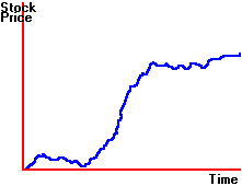
Second, we add a source of randomness to the instantaneous rate of return that has statistical properties that capture the fact that observed stock prices vary, and that a typical stock price path has variance that increases with time. An example is displayed in Figure 6.1.

Figure 6.1

Stock Price Dynamics with Uncertainty

Black and Scholes assume a model for stock price dynamics that is formally described as geometric Brownian motion (see Appendix D, topic D.5, Distribution of Stock Prices). This model has the following form:

Here there are two factors that affect the instantaneous rate of return on a stock. The first is time. Over the "period" of time dt, the stock's return changes by the amount mdt. The second factor is uncertainty. This is illustrated graphically in Figure 6.2.

Figure 6.2

Stock Price as a Function of Time

The straight line shows you the continuously compounded growth of a stock price in the certainty model. The wandering line shows you the effect of adding one source of uncertainty to the certainty model. The sensitivity to this source of uncertainty is captured by the term s which is the volatility coefficient for the stock price. The net effect of adding the term sdz to the certainty model is to create a "noisy" or "stochastic" path for stock prices around the certainty path. The drift for the uncertainty model is the “instantaneous return” not the continuously compounded return. The reason for making such a distinction is that the logarithm of the instantaneous stock return has a volatility adjusted drift as derived in technical appendix D.6 Distribution of Stock Prices.

Uncertainty in the model is added to let the model better satisfy properties exhibited by real world stock prices. These properties are described in the next section and their mathematical representations are formally presented in Appendix D, topic D.5, Distribution of Stock Prices.

Properties of the Volatility Term

You may have observed that not only are stock prices volatile, but the longer the period of time in question, the greater the total price variance. Figure 6.3 illustrates this for the automobile manufacturers, GM and Chrysler.

Figure 6.3

GM & Chrysler Stock Price Graphs

You can see that prices tend to be less volatile over short periods of time, and the total variability of prices increases with the length of the time period. In the geometric Brownian motion model of stock prices, this characteristic of stock prices is captured by the assumptions made on random variable, z.

These properties are:

1. The change in z is the product of a standard normal random variable (i.e., with mean zero and standard deviation 1), and the square root of the interval of time. This implies that the variance of stock prices increases linearly with time.

2. For any two (non overlapping and small) intervals of time, the change in z is independent. This is consistent with the (weak form of the) efficient markets hypothesis.

These assumptions, together with the equation describing the stock price process, give a nice distribution for the stock price. That is, the random variable log(ST)-log(S), which is the change in the stock price between now and period T, is normally distributed with mean (m - s2/2)T and variance s2T. As a result, S has a lognormal distribution as below:

and the variance of ST is:

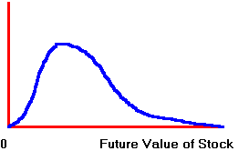
The lognormal distribution has the general shape shown in Figure 6.4.

Figure 6.4

Lognormal Probability Distribution

As you can see, the lognormal distribution preserves the "limited liability" nature of a stock, which means that the stock price can never be negative.

Now that we have a well defined stock price process, we can go on to value options. This is done in the next topic The Black-Scholes Option Pricing Model.

previous topic

next topic