![]() 3.7
Two-Period Asian Option Example
3.7
Two-Period Asian Option Example
You
can apply the binomial model to value non-standard
options. The options we will now
consider are Asian options. The payoff at maturity for an Asian
call is max {Sa - X,0}
where Sa
is
the average stock price over the life
of the option. This option may be
attractive to firms that wish to hedge a stream of transactions over time.
This is because the average price risk becomes a more relevant factor
than the price at one time.
Defining
the underlying asset in this way greatly complicates the option valuation
problem. Now, its value depends
upon the path followed by the underlying asset, and thus it is a path-dependent option. Note
that the problem is not to determine the option value at the end of its life,
but rather at the beginning, when we do not know which path the stock price will
take.
The
beauty of the binomial approach is that the same principles (i.e., riskless
hedge, or synthetic option) still apply and provide a way to calculate the value
of the option. The difference is
that the tree diagram becomes more complex.
Consider
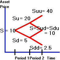
the tree in Figure 3.12 for the underlying stock price.
Figure 3.12
Binomial Tree for Stock Prices

To
value an Asian option we first calculate the average stock price at every node. To simplify this calculation we make the assumption that the
average price is calculated only after the first tick is realized (i.e.,
starting after the end of period 1). Thus,
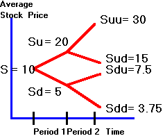
if there is an uptick in period 1, then Su = 20 but Suu = (20 +
40)/2 where now Su, Suu etc., refer to the average stock price process.
The
tree in Figure 3.13 shows you the average prices after making these simplifying
assumptions. We preserve the first
part of the tree, and replace the terminal nodes with averages.
Calculated with our simplifications, the average price at the lowest node
at the end of period 2 is (5+2.5)/2 = 3.75.
Figure 3.13
Binomial Tree for Average Stock Prices

The
risk-neutral probabilities remain the same (i.e., 0.34, 0.66 for an uptick and
downtick, respectively). You can
now apply the risk-neutral valuation principle as before.
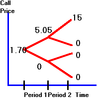
You can verify that the value of the call option is obtained as shown in
Figure 3.14.
Figure 3.14
Call Option Value

The
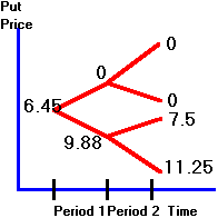
put option can be valued in the same way. The
tree diagram for the put option is as shown in Figure 3.15.
Figure 3.15
Put Option Value

Next,
Chapter 4 introduces you to the use of options for controlling risk by applying
the principle of dynamic hedging. An
overview of this chapter is provided next in Dynamic
Hedging Strategies.
(C) Copyright 1999, OS
Financial Trading System